The non relativistic Hydrogen atom

The time independant Schrödinger equation

The hydrogen atom is constituted of two particles, one proton and one electron. As we want to solve it using quantum mechanics, we will need to use the Schrödinger equation

\begin{equation} \label{eq:sch} \hat{H} \Psi(\vec{r}) = E \Psi(\vec{r}) \end{equation}

In \eqref{eq:sch} the \( \hat{H} \) is the Hamiltonian of the system and can be expressed as the sum of three operators.

\begin{equation} \label{eq:operators} \hat{H} = \hat{T}_{e} + \hat{T}_{p} + \hat{V} \end{equation}

Where \( \hat{T} \) is the kinetic energy operator, we can modify the kinetic energy operators to have only one operator depending on the reduced mass of the system \( \mu = \frac{m_em_p}{m_e+m_p} \)

\begin{align} \hat{T}_E + \hat{T}_p &= -\frac{\hbar}{2m_{e}} \nabla^2 - \frac{\hbar}{2m_{p}} \nabla^2 \\ &= -\frac{\hbar}{2} \left[ \frac{1}{m_e} + \frac{1}{m_p} \right] \nabla^2 \\ &= -\frac{\hbar}{2} \frac{m_e + m_p}{m_em_p} \nabla^2 \\ &= - \frac{\hbar}{2 \mu}\nabla^2 \end{align}

And \( \hat{V} \) is the potential operator, here we will study free hydrogen atom, so the only potential is the potential of the proton on the neutron which is described by a Coulomb potential.

\begin{equation} \label{eq:coulomb} \hat{V} = - \frac{Ze^2}{4 \pi \varepsilon_0 r} \end{equation}

In \eqref{eq:coulomb} the \( Z \) is the charge of the nucleus, 1 for the Hydrogen atom, $e$ is the elementary charge (\( e = 1.602176634 \times 10^{-19}\) C),\( \varepsilon_0 \) is the vacuum permittivity (\( \varepsilon_0 = 8.8541878128 \times 10^{-12} \) F.m\(^{-1}\) ) and \(r\) is the distance between the electron and the proton.

\eqref{eq:sch} can then be rewritten for this system

\begin{equation} \label{eq:sch2} \left[ - \frac{\hbar}{2\mu}\nabla^2 - \frac{e^2}{4\pi \varepsilon_0 r} - E \right] \Psi(\vec{r}) = 0 \end{equation}

\( \nabla^2 \) is the Laplacian operator, in spherical coordinates it is \eqref{eq:laplacian}

\begin{equation} \label{eq:laplacian} \nabla^2 = \frac{1}{r^2} \frac{\partial}{\partial r} \left( r^2 \frac{\partial}{\partial r} \right) + \frac{1}{r^2 \sin \theta} \frac{\partial}{\partial \theta} \left( \sin \theta \frac{\partial}{\partial \theta} \right) + \frac{1}{r^2 \sin^2 \theta} \frac{\partial^2}{\partial \Phi^2} \end{equation}

\( \Psi(\vec{r}) \) is the wavefunction of the system, and \( |\Psi(\vec{r})|^2 \) is the probability of finding the electron at the position \( \vec{r} \) (when the origin is the position of the nucleus). This means that the wavefunction needs to be normalized \eqref{eq:normalized}

\begin{equation} \label{eq:normalized} \int_{0}^{+\infty}\int_{0}^{\pi}\int_{0}^{2 \pi} |\Psi(r,\theta,\phi)|^2 r^2 \cos \theta dr d\theta d\phi = 1 \end{equation}

We can now mix \eqref{eq:laplacian} with \eqref{eq:sch2}, we have \eqref{eq:sch3}

\begin{equation} \scriptsize{ \label{eq:sch3} - \frac{\hbar}{2\mu} \left[\frac{1}{r^2} \frac{\partial }{\partial r} \left( r^2 \frac{\partial \Psi(r,\theta,\phi)}{\partial r} \right) + \frac{1}{r^2 \sin \theta} \frac{\partial}{\partial \theta} \left( \sin \theta \frac{\partial\Psi(r,\theta,\phi)}{\partial \theta} \right) + \frac{1}{r^2 \sin^2 \theta} \frac{\partial^2\Psi(r,\theta,\phi)}{\partial \phi^2}  \right] - \frac{e^2}{4\pi \varepsilon_0 r}\Psi(r,\theta,\phi) - E \Psi(r,\theta,\phi) = 0} \end{equation}

We can now drop the minus sign, multiply by \( \frac{2\mu}{\hbar^2} \) and factorize the two last term by \( \Psi(r,\theta,\phi) \)

\begin{equation} \scriptsize{ \label{eq:sch4} \frac{1}{r^2} \frac{\partial }{\partial r} \left( r^2 \frac{\partial \Psi(r,\theta,\phi)}{\partial r} \right) + \frac{1}{r^2 \sin \theta} \frac{\partial}{\partial \theta} \left( \sin \theta \frac{\partial\Psi(r,\theta,\phi)}{\partial \theta} \right) + \frac{1}{r^2 \sin^2 \theta} \frac{\partial^2\Psi(r,\theta,\phi)}{\partial \phi^2}   + \frac{2\mu}{\hbar^2}\left( \frac{e^2}{4\pi \varepsilon_0 r} + E \right) \Psi(r,\theta,\phi) = 0} \end{equation}

Separation of variables

Let’s assume that \( \Psi(r, \theta, \phi) \) is the product of two functions, one that only depends on \( r \) and the other that only depends on \( \theta \) and \( \phi \)

\begin{equation} \label{eq:psi} \Psi(r,\theta,\phi) = R(r)Y(\theta,\phi) \end{equation}

It is now possible to plug \eqref{eq:psi} in \eqref{eq:sch4} and rearrange a bit.

\begin{align} \scriptsize{\frac{Y(\theta,\phi)}{r^2} \frac{\partial }{\partial r} \left( r^2 \frac{\partial R(r)}{\partial r} \right) + \frac{R(r)}{r^2 \sin \theta} \frac{\partial}{\partial \theta} \left( \sin \theta \frac{\partial Y(\theta,\phi)}{\partial \theta} \right) + \frac{R(r)}{r^2 \sin^2 \theta} \frac{\partial^2Y(\theta,\phi)}{\partial \phi^2} + \frac{2\mu}{\hbar^2} \left(\frac{e^2}{4\pi \varepsilon_0 r} + E \right) R(r) Y(\theta,\phi)}&= 0 \\ \label{eq:sch5} \scriptsize{\color{#235FA4}{\frac{1}{R(r)} \frac{\partial }{\partial r} \left( r^2 \frac{\partial R(r)}{\partial r} \right)+ \frac{2\mu r^2}{\hbar^2} \left(\frac{e^2}{4\pi \varepsilon_0 r} + E \right)}} +\color{#FF4242}{ \frac{1}{Y(\theta,\phi) \sin \theta} \frac{\partial}{\partial \theta} \left( \sin \theta \frac{\partial Y(\theta,\phi)}{\partial \theta} \right) + \frac{1}{Y(\phi,\theta) \sin^2 \theta} \frac{\partial^2Y(\theta,\phi)}{\partial \phi^2}} &= 0 \end{align}

In \eqref{eq:sch5} there are two different part, one that only depends on \( r \) (blue) and the other that depends on $\theta$ and \( \phi \) (red). It is then possible to separate this equation in two equation, the radial equation (that depends only on \( r \)) and the angular equation (that depends on \( \phi \) and \( \theta \) ), where \( A \) is a constant.

\begin{align} \label{eq:radial} \frac{d}{d r} \left(r^2 \frac{d R(r)}{d r} \right) + \frac{2\mu r^2}{\hbar^2} \left( \frac{e^2}{4\pi\varepsilon r} + E \right)R(r) - AR(r) &= 0 \\ \label{eq:polar} \frac{1}{\sin \theta} \frac{\partial}{\partial \theta} \left(\sin \theta \frac{\partial Y(\theta,\phi)}{\partial \theta}\right) + \frac{1}{\sin^2 \theta} \frac{\partial^2 Y(\theta,\phi)}{\partial \phi^2} + AY(\theta,\phi) &= 0 \end{align}

The polar equation

The polar equation \eqref{eq:polar} can be separated again, assuming that \( Y(\theta,\phi) \) is the product of two independant functions of \( \theta \) and \( \phi \)

\begin{equation} \label{eq:sepolar} Y(\theta,\phi) = \Theta(\theta)\Phi(\phi) \end{equation}

\eqref{eq:sepolar} can be inserted in \eqref{eq:polar} which gives \eqref{eq:seppolar}

\begin{align} \frac{\Phi(\phi)}{\sin \theta} \frac{d}{d\theta} \left(\sin \theta \frac{d\Theta(\theta)}{d \theta} \right) + \frac{\Theta(\theta)}{\sin^2 \theta} \frac{d^2 \Phi(\phi)}{d \phi^2} + A \Theta(\theta) \Phi(\phi) &= 0 \\ \label{eq:seppolar} \color{#6FDE64}{\frac{\sin \theta}{\Theta(\theta)} \frac{d}{d\theta}\left(\sin \theta \frac{d \Theta(\theta)}{d \theta} \right)} + \color{#FF934F}{\frac{1}{\Phi(\phi)} \frac{d^2 \Phi(\phi)}{d\Phi^2}} + \color{#6FDE64}{A  \sin^2 \theta} &= 0 \\ \end{align}

In \eqref{eq:seppolar} we can see that there are two different parts, one depending only on $\phi$ and the other depending only on $\theta$.

\begin{align} \label{eq:azimuth} \frac{d^2 \Phi(\phi)}{d \phi^2} + B \Phi(\phi) &= 0 \\ \label{eq:plar} \sin \theta \frac{d}{d\theta}\left( \sin \theta \frac{d \Theta(\theta)}{d \theta} \right) + A\sin \theta - B \Theta(\theta) &= 0 \end{align}

\eqref{eq:azimuth} is called the Azimuthal equation, as \( \phi \) descibe the elevation to the plane \( xOy \), and \eqref{eq:plar} is called the Polar equation as \( \theta \) describe the polar angle in the plane \( xOy \)

The Azimuthal equation

The Azimuthal equation \label{eq:azimuth} is a second order differential equation with constant coefficient so its solutions are simply \eqref{eq:azsol}

\begin{equation} \label{eq:azsol} \Phi(\phi) = \alpha e^{im\phi} + \beta e^{-im\phi} \end{equation}

With \( B = m^2\) , m needs to be an integer because \( \Phi(2\pi) = \Phi(0) \) . We can conveniently decide to set \( \beta \) to 0, which gives \eqref{eq:azisol}

\begin{equation} \label{eq:azisol} \Phi(\phi) = \alpha e^{im\phi} \end{equation}

The Polar equation

We can use the fact that \( B = m^2 \) to rewrite and rearrange the Polar equation as \eqref{eq:plar2}

\begin{equation} \label{eq:plar2} \frac{1}{\sin \theta} \frac{d}{d\theta}\left( \sin \theta \frac{d \Theta(\theta)}{d \theta} \right) + \Theta(\theta)\left(A - \frac{m^2}{\sin^2 \theta} \right) = 0 \end{equation}

We will now need to use a change of variables. We will express this equation as a function of \( \cos \theta \). \( P(\cos \theta) = \Theta(\theta)\), we have \( \frac{d}{d \theta} = \frac{d \cos \theta}{d \theta} \frac{d}{d\cos \theta} = -\sin \theta \frac{d}{d \cos \theta} \). Using that, we have \eqref{eq:change1}.

\begin{align} \frac{1}{\sin \theta}\sin \theta \frac{d}{d \cos \theta} \left( \sin^2 \theta \frac{d P(\cos \theta)}{d \cos \theta} \right) + P(\cos \theta) \left(A - \frac{m^2}{\sin^2 \theta} \right) &= 0 \\ \frac{d}{d \cos\theta} \left((1-\cos^2 \theta) \frac{d P(\cos \theta)}{d \cos \theta} \right) + P(\cos \theta) \left( A - \frac{m^2}{1- \cos^2 \theta} \right) &= 0 \\ (1-\cos^2 \theta) \frac{d^2 P(\cos \theta)}{d \cos \theta^2} - 2 \cos \theta \frac{d P(\cos \theta)}{d \theta} + P(\cos \theta)\left(A - \frac{m^2}{1-\cos^2 \theta}\right) \label{eq:change1} \end{align}

\eqref{eq:change1} is a second order differential equation with non-constant coefficient. It has the form of the associated Legendre differential equation where we identify \( A = l(l+1) \) where $l$ is an integer. This solution impose \( 0 \le m \le l\).

\begin{equation} \label{eq:leg} P(\cos \theta) = P_l^{|m|}(\cos \theta) \end{equation}

The spherical harmonics

We can now use \eqref{eq:leg} and \eqref{eq:azisol} to write the general form of \( Y(\theta,\phi) \)

\begin{equation} \label{eq:spheharm} Y_l^m(\theta,\phi) = \alpha e^{im\phi}P_l^{|m|}(\cos\theta) \end{equation}

\( Y_l^m(\theta,\phi) \) needs to be normalized, so we can find the value of \( \alpha \) using the orthonogonality of the associated Legendre polynomials.

\begin{align} \int_0^{\pi} \int_0^{2\pi} Y_l^{m*}(\theta,\phi) Y_l^m(\theta,\phi) \sin \theta d\theta d\phi &= 1 \\ \alpha^2 \int_0^{\pi} \int_0^{2\pi} e^{i(m-m)\phi} P_l^{|m|}(\cos \theta) P_l^{|m|}(\cos \theta) \sin \theta d\theta d\phi&= 1 \\ \alpha^2 \left[\int_0^{2\pi} d\phi\right] \left[\int_{0}^{\cos \pi} \theta P_l^{|m|}(\cos \theta) P_l^{|m|}(\cos\theta) \sin \theta d\theta \right] &= 1 \\ \alpha^2 \frac{4\pi(l+|m|)!}{(2l+1)(l-|m|)!} &= 1 \\ \alpha &= \sqrt{\frac{2l+1}{4\pi}\frac{(l-|m|)!}{(l+|m|)!}} \\ \label{eq:spheharmnorm} \end{align}

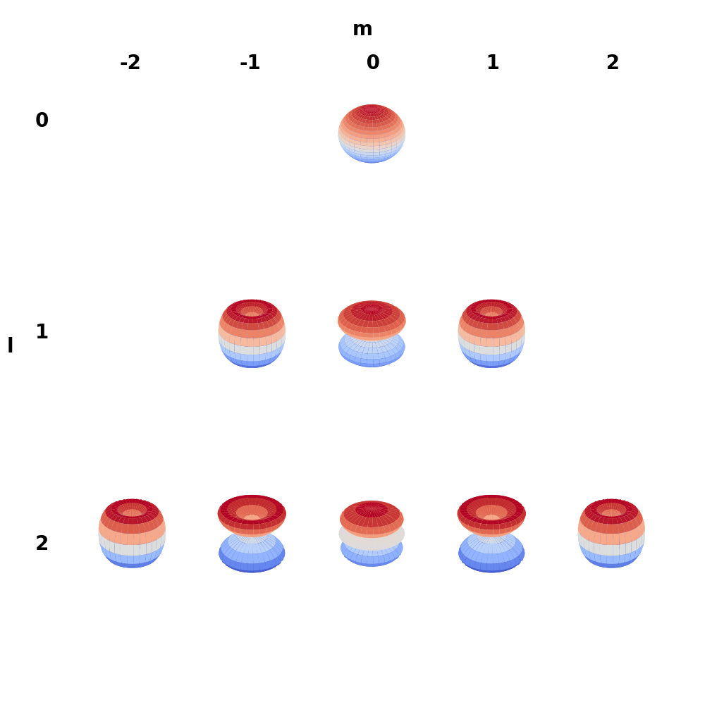
We now have a general formula for \( Y_l^m(\theta,\phi) \), which is called a spherical harmonic \eqref{eq:sphericalharmonic}. Due to the Legendre polynomials orthogonality, all the spherical harmonics are orthogonals.

\begin{equation} \label{eq:sphericalharmonic} Y_l^m(\theta,\phi) = \sqrt{\frac{2l+1}{4\pi}\frac{(l-|m|)!}{(l+|m|)!}}e^{im\phi} P_l^{|m|}(\cos \theta) \end{equation}

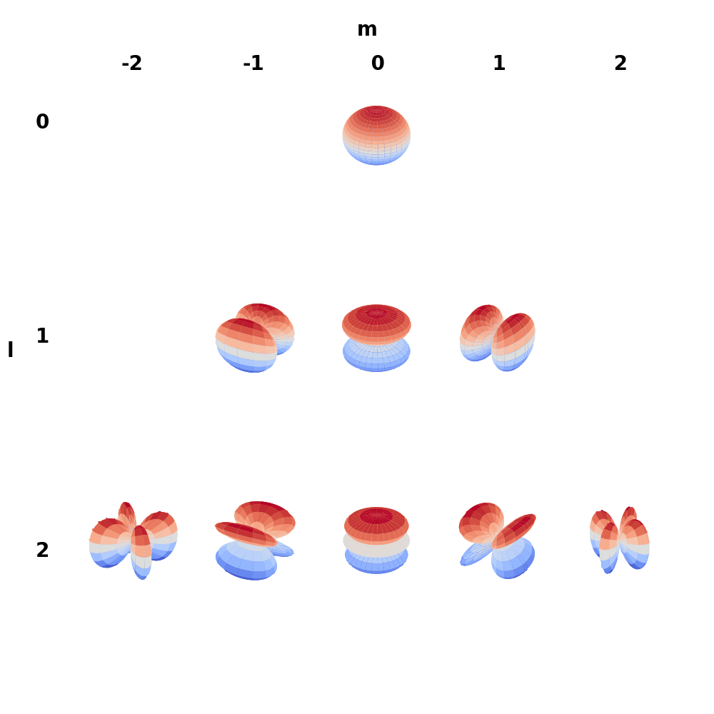
In order to deal with purely real functions, it is common to use the real spherical harmonics which can be obtained by a simple linear combination of the complex spherical harmonics \eqref{eq:ctor}

\begin{equation} \label{eq:ctor} \tilde{Y}_l^m = \begin{cases} \frac{(-1)^m}{\sqrt{2}} \left( Y_l^m + Y_l^{m\dagger} \right) & \mbox{if } m > 0 \\ Y_l^m & \mbox{if } m = 0 \\ \frac{(-1)^m}{i\sqrt{2}} \left( Y_l^{m} - Y_l^{m\dagger} \right) & \mbox{if } m < 0 \end{cases} \end{equation}

The radial equation

The radial equation is trickier to solve, first we need to plug the value of \( A \) found in \eqref{eq:change1}.

\begin{equation} \label{eq:rad1} \frac{d}{dr}\left( r^2 \frac{dR(r)}{dr} \right) + \frac{2\mu r^2}{\hbar^2} \left( \frac{e^2}{4\pi \varepsilon_0 r} + E \right)R(r) - l(l+1)R(r) = 0 \end{equation}

We will now make a first change of variables, we will use a function \( u(r) \) such that \( R(r) = \frac{u(r)}{r} \).

\begin{align} \nonumber \frac{d}{dr} \left( r^2 \frac{dR(r)}{dr} \right) &= \frac{d}{dr} \left(r \frac{d u(r)}{dr} - u(r) \right) \\ \nonumber &= \frac{du(r)}{dr} - \frac{du(r)}{dr} + r\frac{d^2u(r)}{dr^2} \\ \label{eq:rad2} &= r\frac{d^2 u(r)}{dr^2} \end{align}

Using \eqref{eq:rad2} we can rewrite \eqref{eq:rad1} as \eqref{eq:rad3} and make some rearangements

\begin{align} r \frac{d^2 u(r)}{dr^2} + \frac{2\mu}{\hbar^2} \left(\frac{e^2}{4\pi\varepsilon_0 r} + E \right)ru(r) - \frac{l(l+1)}{r} u(r) &= 0 \\ -\frac{\hbar^2}{2\mu}\frac{d^2 u(r)}{dr^2} - \frac{e^2}{4\pi\varepsilon_0 r}u(r) - Eu(r) + \frac{\hbar^2}{2\mu}l(l+1) \frac{u(r)}{r^2} &= 0 \\ -\frac{\hbar^2}{2\mu}\frac{d^2 u(r)}{dr^2} + u(r) \left(-\frac{e^2}{4\pi\varepsilon_0 r} + \frac{\hbar^2}{2\mu}\frac{l(l+1)}{r^2}\right) &= Eu(r) \\ \label{eq:rad3} -\frac{\hbar^2}{2\mu E}\frac{d^2 u(r)}{dr^2} + u(r) \left(-\frac{e^2}{4\pi\varepsilon_0 r E} + \frac{\hbar^2}{2\mu E}\frac{l(l+1)}{r^2}\right) &= u(r) \end{align}

It is now convenient to use a new variable \( k^2 = -\frac{2\mu E}{\hbar^2} \), it will simplify the notation. \eqref{eq:rad3} is now \eqref{eq:rad4}

\begin{align} \nonumber \frac{1}{k^2}\frac{d^2 u(r)}{dr^2} + u(r) \left(-\frac{e^2}{4\pi\varepsilon_0 r E} - \frac{1}{k^2}\frac{l(l+1)}{r^2}\right) &= u(r) \\ \label{eq:rad4} \frac{1}{k^2}\frac{d^2 u(r)}{dr^2} &= u(r) \left(\frac{1}{k^2} \frac{l(l+1)}{r^2} + 1 - \frac{\mu e^2}{2\pi \varepsilon_0 \hbar^2 k} \frac{1}{kr} \right) \\ \end{align}

It is time for a second change of variable, we will use \( \rho = 2kr \), now \( u(r) \) is \( w(\rho) \) and \( 2k dr = d\rho\). We will also introduce the quantity \( \rho_0 = \frac{\mu e^2}{2\pi \varepsilon \hbar^2 k} \) which will again simplify the notation. We can rewrite \eqref{eq:rad4} as \eqref{eq:rad5}.

\begin{equation} \label{eq:rad5} \frac{d^2 w(\rho)}{d \rho^2} = w(\rho) \left( \color{#235FA4}{\frac{l(l+1)}{\rho^2}} + \color{#FF4242}{\frac{1}{4}} - \frac{\rho_0}{2\rho} \right) \end{equation}

As we still don’t know \( w(\rho) \), we will take a look at its asymptotic behavior for small and large values of \( \rho \) (\( \rho \rightarrow +\infty \) and \( \rho \rightarrow 0 \)).

Limit at \( \rho \rightarrow + \infty \)

For very large values of $\rho$, only the red term of the parenthesis on the right hand side of \eqref{eq:rad5} does not vanish, we can rewrite.

\begin{equation} \label{eq:rad6} \frac{d^2 w_{\infty}(\rho)}{d\rho^2} = \frac{1}{4}w_{\infty}(\rho) \end{equation}

\eqref{eq:rad6} is a second order differential equation with constant coefficients and has a simple solution \eqref{eq:rad7} where A and B are constants.

\begin{equation} \label{eq:rad7} w_{\infty}(\rho) = A e^{\frac{1}{2}\rho} + B e^{-\frac{1}{2}\rho} \end{equation}

As our solution needs to be normalized we have to set \( A=0 \). We will also drop the $B$ for the moment and compute the normalization constant at the end. We now have our solution \eqref{eq:rad8}

\begin{equation} \label{eq:rad8} w_{\infty}(\rho) = e^{-\frac{1}{2}\rho} \end{equation}

Limit at $\rho \rightarrow 0$

For very small values of $\rho$, the blue term in the parenthesis of \eqref{eq:rad5} will dominate the other terms and we can rewrite the equation

\begin{equation} \label{eq:rad9} \frac{d^2 w_0(\rho)}{d\rho^2} = w_0(\rho) \frac{l(l+1)}{\rho^2} \end{equation}

\eqref{eq:rad9} is again a second order differential equation with constant coefficients and also has a simple solution \eqref{eq:rad10} where C and D are constants.

\begin{equation} \label{eq:rad10} w_0(\rho) = C \rho^{l+1} + D \rho^{-l} \end{equation}

Again with this solution, we have to set \( D=0 \) because we need it to be normalizable. We will drop \( C \) for the moment and include it in the final normalization constant.

\begin{equation} w_0(\rho) = \rho^{l+1} \end{equation}

Now that we have studied the asymptotic behavior of \( w(\rho) \), we can rewrite as a function of these two special functions and include a third one \( v(\rho) \)

\begin{align} \nonumber w(\rho) &= w_0(\rho)w_\infty(\rho)v(\rho) \\ \label{eq:rad11} &= \rho^{l+1}e^{-\frac{1}{2}\rho}v(\rho) \end{align}

We can now insert \eqref{eq:rad11} in \eqref{eq:rad5} and rearrange it.

\begin{align} \scriptsize{\frac{d^2}{d\rho^2} \left(\rho^{l+1}e^{-\frac{1}{2}\rho}v(\rho) \right)} &= \scriptsize{ \rho^{l+1}e^{-\frac{1}{2}\rho}v(\rho)\left(\frac{l(l+1)}{\rho^2} + \frac{1}{4} - \frac{\rho_0}{2\rho} \right)} \\ \scriptsize{\frac{d^2v(\rho)}{d\rho^2} \left[ \rho^{l+1}e^{-\frac{1}{2}\rho} \right] + \frac{d v(\rho)}{d\rho} \left[2(l+1)\rho^le^{-\frac{1}{2}\rho}-\rho^{l+1}e^{-\frac{1}{2}\rho} \right] + v(\rho) \left[\frac{1}{4}\rho^{l+1}e^{-\frac{1}{2}\rho} - (l+1)\rho^le^{-\frac{1}{2}\rho} + l(l+1)\rho^{l-1}e^{-\frac{1}{2}\rho}  \right]} &= \scriptsize{\rho^{l+1}e^{-\frac{1}{2}\rho}v(\rho)\left(\frac{l(l+1)}{\rho^2} + \frac{1}{4} - \frac{\rho_0}{2\rho} \right) } \\ \label{eq:rad12} \frac{d^2v(\rho)}{d\rho^2}\rho + \frac{d v(\rho)}{d\rho}\left[2l+2 -\rho \right] + v(\rho) \left[\frac{\rho_0}{2} - (l+1) \right] &= 0 \end{align}

\eqref{eq:rad12} is now in a form that allows us to solve it using a power serie.

\begin{align} \label{eq:pow1} v(\rho) &= \sum_{j=0}^{\infty} c_j \rho^j \\ \label{eq:pow2} \frac{d v(\rho)}{d\rho} &= \sum_{j=0}^\infty c_j j \rho^{j-1} = \sum_{j=0}^\infty (j+1) c_{j+1} \rho^j \\ \label{eq:pow3} \frac{d^2 v(\rho)}{d\rho^2} &= \sum_{j=0}^\infty j(j+1)c_{j+1} \rho^{j-1} \end{align}

Now we can use \eqref{eq:pow1}, \eqref{eq:pow2} and \eqref{eq:pow3} to rewrite \eqref{eq:rad12}

\begin{align} \rho \sum_{j=0}^\infty j(j+1) c_{j+1} \rho^{j-1} + 2(l+1) \sum_{j=0}^\infty (j+1) c_{j+1} \rho^j - \rho \sum_{j=0}^\infty j c_j \rho^{j-1} + \sum_{j=0}^\infty c_j \rho^j \left[\frac{\rho_0}{2} -(l+1)\right] &= 0\\ \label{eq:pow4} \sum_{j=0}^\infty \rho^j \left[j(j+1)c_{j+1} + 2(l+1)(j+1)c_{j+1} - jc_j + c_j \left(\frac{\rho_0}{2} - (l+1) \right) \right] &= 0 \end{align}

\eqref{eq:pow4} raises the condition that the term in the parenthesis must be equal to 0

\begin{align} c_{j+1} \left[j(j+1) + 2(l+1)(j+1) \right] - c_j \left[j-\frac{\rho_0}{2} + (l+1) \right] &= 0 \\ \label{eq:recur} c_{j+1} &= \frac{j - \frac{\rho_0}{2} + (l+1)}{(j+1)(j+2l+2)} c_j \end{align}

This condition gives us a recurrence relation \eqref{eq:recur} for the coefficients of the power serie.

For very large values of \( j \), we have \( c_{j+1} \approx \frac{j}{j(j+1)} c_j \Rightarrow c_j \approx \frac{1}{j!} \)

If we use this approximation we have that \c v(\rho) \approx \sum_{j=0}^\infty \frac{1}{j!}\rho^j = e^{\rho} \)

With this, \( w(\rho) = \rho^{l+1}e^{\frac{1}{2}\rho} \) which is not normalizable. As this behaviour happens when j goes up to infinity, this means that the serie is bounded, there is a \( j_{max} \)

\begin{align} c_{j_{max}+1} &= 0 \\ \frac{j_{max} - \frac{\rho_0}{2} + l + 1}{(j+1)(j+2l+2)}c_{j_{max}} &= 0 \\ j_{max} - \frac{\rho_0}{2} + l + 1 &= 0 \end{align}

If we use \( n = j_{max}+l+1 \), we have \eqref{eq:n}

\begin{align} \label{eqref:n} n &= \frac{\rho_0}{2} \\ 2n &= \frac{\mu e^2}{2\pi\varepsilon_0\hbar^2k} \\ 2n &= \frac{\mu e^2}{2\pi\varepsilon_0\hbar^2\sqrt{-\frac{2\mu E}{\hbar^2}}} \\ \label{eq:n} E &= -\frac{\mu e^4}{32 \pi^2 \varepsilon_0^2 \hbar^2 n^2} \end{align}

If we simplify all the constants in \eqref{eq:n}, we have the famous equation for the energy levels of the hydrogen atom \( E \approx \frac{-13.6}{n^2}\) eV. This implies that the energy is quantized, defined by the number $n$ which is called the principal quantum number.

The associated Laguerre polynomials are a certain type of polynomials which are solution to the differential equation \eqref{eq:lag1}

\begin{equation} \label{eq:lag1} x \frac{d^2 L_m^\alpha(x)}{dx^2} + (\alpha + 1 - x) \frac{d L_m^\alpha(x)}{d x} + m L_m^\alpha(x) = 0 \end{equation}

If we look at \eqref{eq:rad12} we can identify \( m = n - l - 1 \) and \( \alpha = 2l + 1\) . This has a constaint that \( 0 \le l < n \), we can now write the final formula and change the variables back \eqref{eq:fin1}

\begin{align} w(\rho) &= \rho^{l+1} e^{-\frac{1}{2}\rho} L_{n-l-1}^{2l+1}(\rho) \\ R(\rho) &= \rho^l e^{-\rho/2} L_{n-l-1}^{2l+1}(\rho) \\ \label{eq:fin1} R_{n,l}(r) &= (2kr)^l e^{-kr} L_{n-l-1}^{2l+1}(2kr) \end{align}

The radial function obtained in \eqref{eq:fin1} is however not normalized and we need to multiply it by the correct normalization constant \( N \)

\begin{align} \int_{0}^\infty R^*_{n,l}(r) R_{n,l}(r) r^2 dr &= 1 \\ \int_0^\infty N^2 (2kr)^2l e^{-2kr} \left( L_{n-l-1}^{2l+1}(2kr)\right)^2 r^2 dr &= 1 \\ \end{align}

In order to solve this integral, we need to make one change of variable \( x = 2kr \), which implies \( dx = 2kdr \)

\begin{align} N^2 \int_0^\infty (x)^2l e^{-x} \left( L_{n-l-1}^{2l+1}(x) \right)^2 \frac{x^2}{(2k)^2} \frac{1}{2k} dx &= 1 \\ \label{eq:int1} \frac{N^2}{(2k)^3} \int_0^\infty (x)^{2l+2} e^{-x} \left( L_{n-l-1}^{2l+1} \right)^2 dx &= 1 \end{align}

Thankfully, the integral in \eqref{eq:int1} is known \eqref{eq:int2}

\begin{equation} \label{eq:int2} \int_0^\infty x^{k+1} \left(L_j^k(x) \right)^2 e^{-x} dx = (2j+k+1) \frac{(j+k)!}{j!} \end{equation}

We can insert it in \eqref{eq:int1} and we have

\begin{align} \frac{N^2}{(2k)^3} (2(n-l-1)+(2l+1)+1) \frac{((n-l-1)+(2l+1))!}{(n-l-1)!} &= 1 \\ \frac{N^2}{(2k)^3} 2n \frac{(n+l)!}{(n-l-1)!} &= 1 \\ N &= \sqrt{\frac{(n-l-1)!(2k)^3}{2n(n+l)!}} \end{align}

It is now time to introduce a new constant which has the dimension of a length

\begin{equation} a_\mu = \frac{4\pi \varepsilon_0 \hbar^2}{e^2\mu} \end{equation}

Using \( a_\mu \) we have \( k = \frac{1}{na_\mu} \)

The normalized radial function can now be written \eqref{eq:fin3}

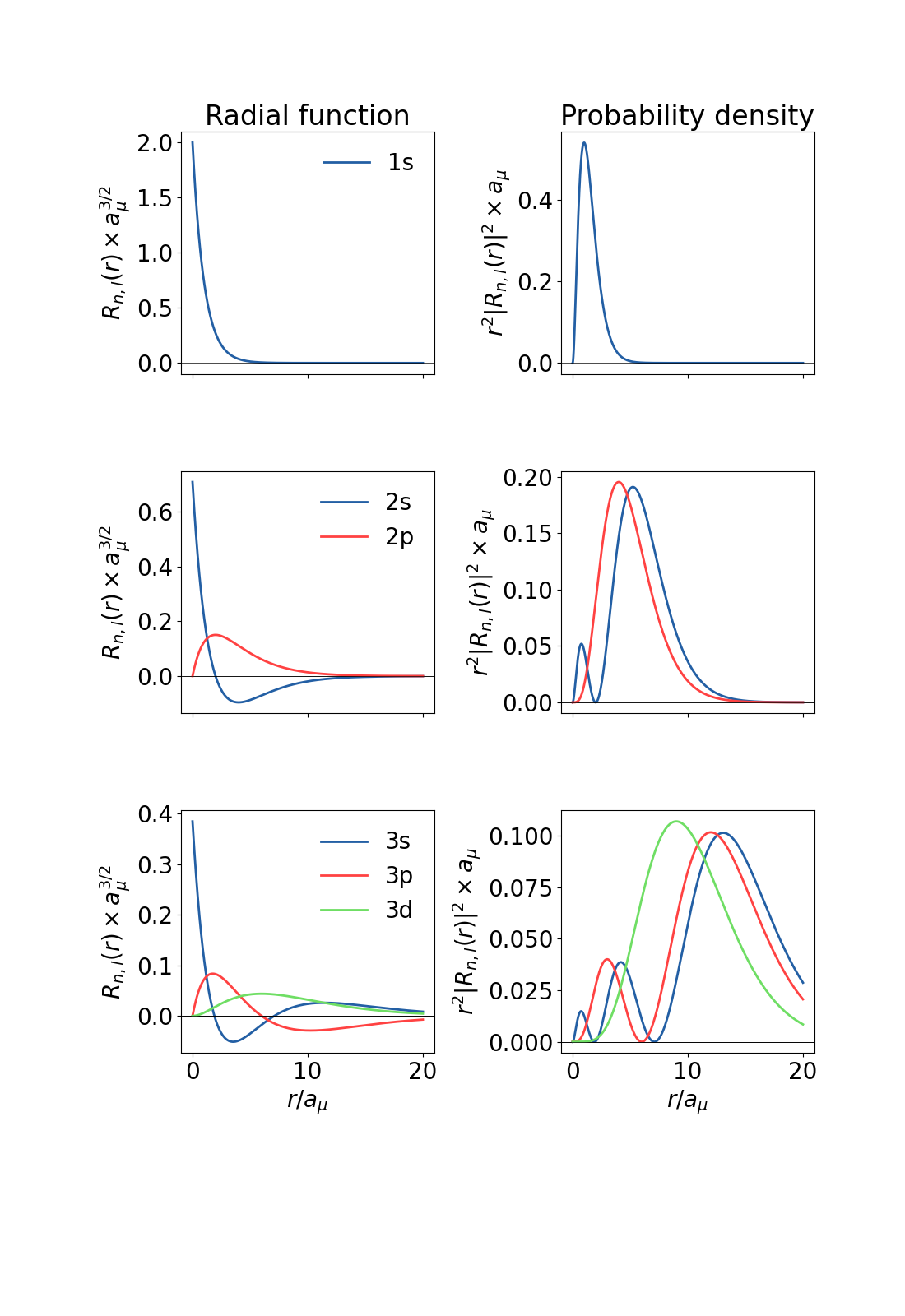
\begin{equation} \label{eq:fin3} R_{n,l}(r) = \sqrt{\frac{(n-l-1)!}{2n(n+l)!}}\left(\frac{2}{na_\mu}\right)^{l+\frac{3}{2}}r^l e^{-\frac{r}{na_\mu}} L_{n-l-1}^{2l+1}\left(\frac{2r}{na_\mu}\right) \end{equation}

The first few functions of this kind are shown

The wavefunction

We have succesfully solved the radial and angular equations, it is now time to put all the results together,using here the real spherical harmonics.

\begin{equation} \Psi_{l,m,n}(r,\theta,\phi) = \sqrt{\frac{(n-l-1)!}{2n(n+l)!}}\left(\frac{2}{na_\mu}\right)^{l+\frac{3}{2}}r^l e^{-\frac{r}{na_\mu}} L_{n-l-1}^{2l+1}\left(\frac{2r}{na_\mu}\right)\tilde{Y}_l^m(\theta,\phi) \end{equation}

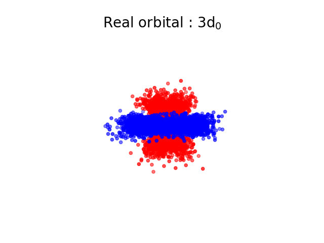
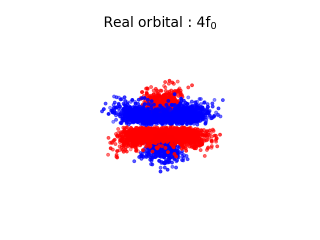
The square of the wavefunction represents the probability of finding the electron at the position \( \vec{r} \), it is possible to use this probability to simulate the fact that we would measure such an electron. If we do it a lot of times, we should get the shape of an “orbital” which represents the electron. In the next images, each point is coloured differently depending on the sign of \( \Psi \).

The energy spectrum

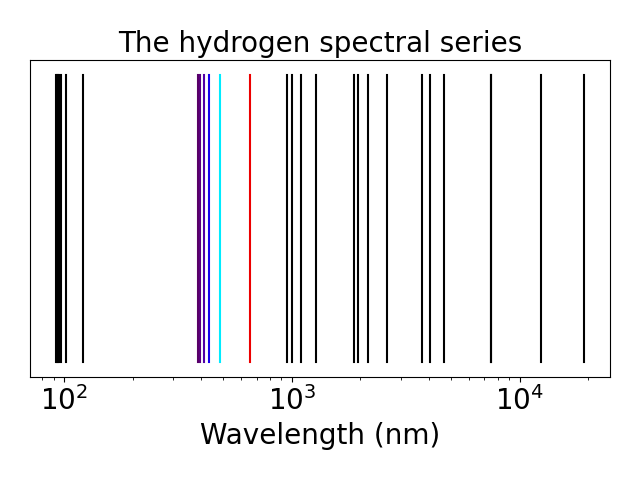
We can use the quantization of the energy \eqref{eq:n} to compute to spectral series of the hydrogen atom. For each value of $n$ we can compute the energy difference with all the other states. This is the energy that we need to give to the atom to go from the first state to the second.

We can see that the energies are grouped. Each group correspond to all the excitations coming from one level to all the others, the first group on the left corresponds to the electron going from the first level to all the others and is called the Lyman series, the second group is called the Balmer series and is the only group that crosses the visible spectrum, the third group is the Paschen series, then the Brackett series, the Pfund series and the Humphreys series.

Code

All the code used to generate the plots in this article can be found on the dedicated GitHub repository.